Marginal Loss Factors (MLFs) are not just a technical detail — they’re a powerful signal about the grid’s strengths and weaknesses. Developers who use them wisely can steer projects toward locations that are not only resource-rich but also financially and system-friendly.
This post is not about explaining every detail of what MLFs are or how they’re calculated in the National Electricity Market (NEM). Instead, the focus is on something more practical: how GIS techniques can unlock the value hidden in MLF data. By visualising and analysing MLFs spatially, we can:
- Pinpoint promising zones for new energy projects,
- Identify early “red flags” that could derail development, and
- Support decisions around where new transmission infrastructure is most needed to improve system performance.
The Big Question Developers Ask: “Where?”
In the energy sector, as in many industries, developers are constantly asking the same question: Where should we build next?
Finding the right site is not just about chasing sunshine or wind — it’s about making sure the location delivers the best possible return on investment. And here’s the challenge: what looks like a great project on paper can quickly become unviable once you factor in network constraints, transmission distances, or poor MLF values.
Without the right methods and tools, developers risk burning through time and money assessing sites that were never suitable to begin with.
My Journey Into GIS
This challenge has shaped my career. At one company I worked for, we received hundreds of property offers from landowners eager to host renewable projects. At first, every site had to be manually reviewed — a process that became overwhelming as numbers grew.
That’s when I turned to GIS tools. By layering data on connection points, transmission capacity, environmental constraints, and MLF values, we were able to rapidly discard unsuitable sites — those that were too far from the grid, in protected areas, or at already saturated connection points.
The impact was huge: not only did our efficiency skyrocket, but we also built an in‑house platform to proactively identify suitable zones ourselves, rather than waiting for opportunities to come to us.
From Practice to Research
These methods didn’t just improve project development — they also became central to my research. In my PhD, I use GIS combined with Multi-Criteria Decision Making (MCDM) techniques to identify optimal locations for deploying electric vehicle (EV) charging infrastructure.
The analysis integrates diverse criteria such as:
- Distribution system hosting capacity,
- Vehicle density and travel patterns,
- Availability of existing amenities,
- Forecasted demand growth.
By balancing these factors spatially, GIS transforms a complex decision into a clear, evidence-based strategy for infrastructure deployment. Figure 1 shows an example of one scenario analysis output.
In the same way, the same approach is applicable to finding suitable locations for new energy projects. Modelling the appropriate criteria and tuning weights correctly can help to pinpoint the best sites, and MLF can be an important criterion to include in the modelling.
Let’s start by addressing what an MLF is first, in simple terms.
Marginal Loss Factors, better known as MLFs, are, in simple terms, indices calculated for connection points across the NEM that point to areas currently experiencing high stress. High stress can be due to loads or generation to the grid, manifested as energy losses.
It is important to emphasise that energy losses are undesirable from a system’s perspective; they do not benefit any stakeholder and, in fact, hinder them, as more energy must be generated to offset those losses. Therefore, AEMO has developed a methodology that adjusts electricity prices at different points of the network to reflect the energy losses involved in transporting electricity across the grid.
In Australia’s electricity market, every region has a Regional Reference Node (RRN). This is the anchor point in the grid that sets the reference price for that region. By default, the RRN is assigned a value of 1.0.
For every other connection point on the grid, the MLF measures the extra electricity lost when power flows between that point and the RRN. Because electricity is lost as heat along transmission lines, the actual energy that reaches the grid is always a little less than what’s generated.
Each connection point gets its own MLF, and these values can vary — even between places that are geographically close — depending on the transmission network around them. Still, we often see clusters of similar MLFs in areas that share the same transmission infrastructure.
MLFs are not static
One important aspect of Marginal Loss Factors is that they are not fixed. MLFs are recalculated every year by AEMO, and they can change significantly from one year to the next. This is especially true in areas of low grid strength, where small changes in network flows or the addition of a new project can have a disproportionate effect on losses. For developers and investors, this means that a project’s financial performance may vary year-to-year based not only on weather and market prices, but also on shifts in its MLF. In extreme cases, a generation project that once enjoyed an MLF above 1.0 (boosting revenue) might see it fall below 1.0, resulting in a reduction of revenues.
Facility-specific factors
Another subtlety is that MLFs are calculated on the basis of each facility’s individual energy flows. This means that two facilities located side by side can end up with different MLF values. It often comes as a surprise to developers that neighbouring projects, using the same transmission line, can experience different financial outcomes simply due to their connection arrangements, load profiles, or the way the network models their flows.
The role of regional balance
Ultimately, MLFs reflect the balance between supply and demand within a region. When supply and demand are well matched, losses are minimised, and MLFs are higher. When the balance is skewed — for example, when a region has far more generation than local demand — losses increase as electricity is pushed long distances through the network, and MLFs fall.
A good example is in Central Queensland. The Boyne Smelter, one of Australia’s largest single electricity users, benefits from a <1 MLF (currently 0.9621 in the latest release) because it sits near a large source of local generation at Gladstone Power Station. However, when Gladstone shuts down, that balance will change. Without local generation to match its load, more power will need to travel longer distances to supply the smelter, and its MLF is expected to increase (probably >1). This illustrates how closely tied MLFs are to the evolving structure of the grid, and why they must be re-evaluated each year.
How can we make use of MLFs in project development?
As mentioned earlier, MLFs tend to be similar for nearby connection points, except in cases where the network topology creates sharp differences. This means that with the right data and GIS tools, it’s possible to quickly identify zones of relatively high or low MLFs across the grid.
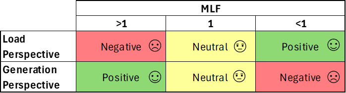
From a project development perspective, understanding MLFs is critical because they directly affect the financial performance of an energy asset:
- High MLF areas (>1.0): These zones are attractive for generation projects (solar farms, wind farms, batteries) because each unit of electricity injected into the grid is effectively worth more. Locating in a high-MLF region means your project is rewarded financially, since it reduces system losses and delivers extra value to the market.
- Low MLF areas (<1.0): Here, generators are penalised because every MWh produced is discounted. On the other hand, these locations can be attractive for demand-side projects (industrial loads, hydrogen electrolysers, datacentres). Consuming electricity in a low-MLF area helps the grid by reducing transmission losses, so it can sometimes come with price advantages or system benefits.
Strategic use of MLFs
- Site selection
Overlay MLF maps with resource maps (e.g., solar irradiation, wind speeds) to find the sweet spots where good resource quality meets strong grid economics. - Technology choice
- High-MLF zones favour generation assets.
- Low-MLF zones may favour loads or storage, which can take advantage of being rewarded as demand.
- Grid negotiation
Early awareness of MLFs helps in discussions with network service providers. A project in a low-MLF area may need stronger justification or complementary grid benefits to be viable. - Portfolio balance
Large developers often spread assets across different regions. Factoring in MLFs helps balance risks — avoiding clustering all projects in areas prone to low or volatile loss factors.
Why it matters for developers
MLFs can make or break the economics of a project:
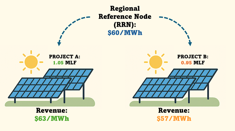
- A solar farm earning $60/MWh with an MLF of 0.95 effectively gets only $57/MWh.
- The same project with an MLF of 1.05 would receive $63/MWh.
That 10% swing can mean millions of dollars over a project’s lifetime — enough to determine whether a project gets financed (See image Figure 2).
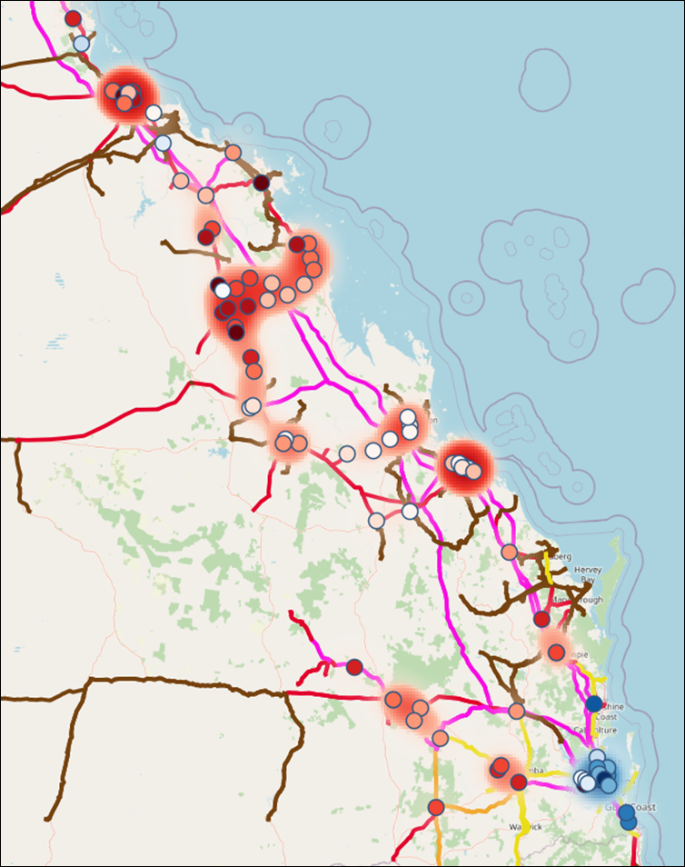
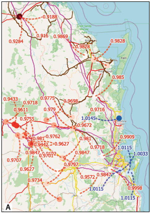
In the image below (Figure 3) an example of the distribution of MLFs across QLD is presented.
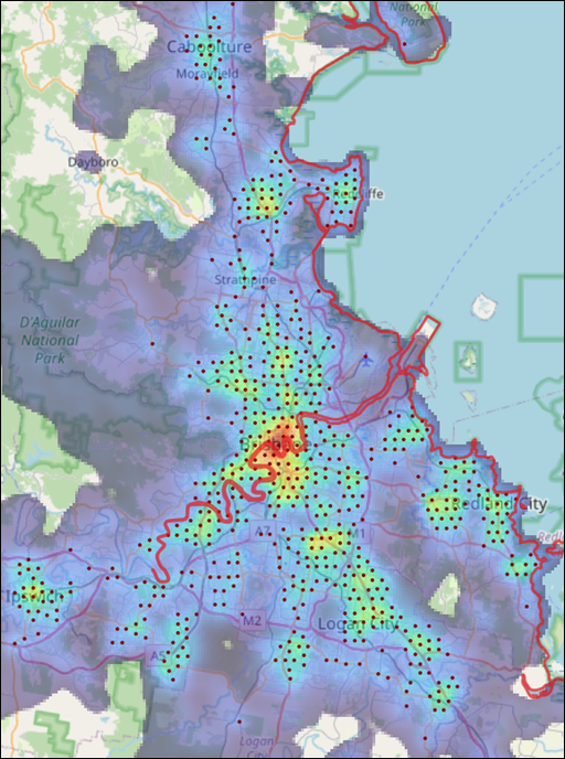
A more general and sometimes useful manner to present the MLFs to identify “hub” is in heatmaps, as in the figure below (Figure 4).

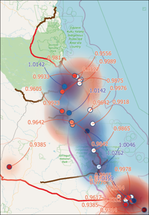
The figure above shows hubs where low or high MLFs can be identified. But as mentioned before, each specific case must be analysed carefully, as there are instances where MLFs can be diametrically different in proximity. As an example, the figure below (Figure 5) shows that the upper part of the QLD NEM presents overlapping of MLFs >1 and <1 in a relatively close distance.
Nevertheless, identifying MLFs hub is still a valuable piece of information to understand potential positive or negative impacts for a new project.
Key takeaways
MLFs change from year to year and can change significantly (particularly in areas of low grid strength).
MLFs are generated on the basis of each facility’s individual energy flows – facilities next to each other can have different MLFs. Generally, loads are higher than generators.
Balancing regional supply and demand improves MLFs. Expect, for example, the MLF for Boyne Smelter (2024–25 MLF = 0.9621) to increase when Gladstone Power Station shuts down.